Project-EDA and Model Building for loan prediction app

This is a very popular project for hands on practice. Here I have applied couple of methods to improve the performance of this model.

Let’s c what can we do with this data set.

Load the data set

Loading the training and test data set locally.

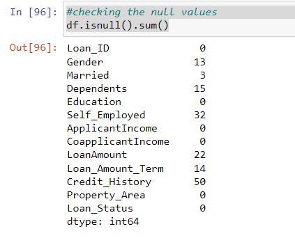
Check for null values

As you can se we are getting null values for many of the columns, which are both numerical and categorical. Let’s handle the numerical value first.

Handling the null values for numerical columns

There are many method for handling null value but the easy one is filling the particular cell with the mean value of the column. Mean depicts the number which has majority so it could be replaced for the null values.

df['ApplicantIncome'] = df['ApplicantIncome'].fillna(df['ApplicantIncome'].mean())
df['CoapplicantIncome'] = df['ApplicantIncome'].fillna(df['ApplicantIncome'].mean())
df['LoanAmount'] = df['ApplicantIncome'].fillna(df['ApplicantIncome'].mean())
df['Loan_Amount_Term'] = df['ApplicantIncome'].fillna(df['ApplicantIncome'].mean())
df['Credit_History'] = df['Credit_History'].fillna(df['ApplicantIncome'].mean())

Check for duplicate values

In my case, there were no duplicate values.

Checking the outliers

If you do a box plot of the numerical columns, you would see tons of outliers. But graphs can be misleading sometimes, so I decided to compute the outliers. Below is the code for the IQR method..

outliers = []
def detect_outliers_iqr(df):
    data = sorted(df)
    q1 = np.percentile(df, 25)
    q3 = np.percentile(df, 75)
    # print(q1, q3)
    IQR = q3-q1
    lwr_bound = q1-(1.5*IQR)
    upr_bound = q3+(1.5*IQR)
    # print(lwr_bound, upr_bound)
    for i in data: 
        if (i<lwr_bound or i>upr_bound):
            outliers.append(i)
    return outliers# Driver code
columns_outliers = ["ApplicantIncome", "CoapplicantIncome", "LoanAmount", "Loan_Amount_Term","Credit_History"]
sample_outliers_ai = detect_outliers_iqr(df["ApplicantIncome"])
print("Outliers from IQR method: ", sample_outliers_ai)

print("////////////////////////////////////////////////")

sample_outliers_ac = detect_outliers_iqr(df["CoapplicantIncome"])
print("Outliers from IQR method: ", sample_outliers_ac)
print("////////////////////////////////////////////////")
sample_outliers_al = detect_outliers_iqr(df["LoanAmount"])
print("Outliers from IQR method: ", sample_outliers_al)
print("////////////////////////////////////////////////")
sample_outliers_at = detect_outliers_iqr(df["Loan_Amount_Term"])
print("Outliers from IQR method: ", sample_outliers_at)
print("////////////////////////////////////////////////")
sample_outliers_ac = detect_outliers_iqr(df["Credit_History"])
print("Outliers from IQR method: ", sample_outliers_ac)

Plotting the numerical columns to see the skewness

Included in the process of getting rid of the outliers, I plotted the distplot to see the skewness.

import warnings
import matplotlib.pyplot as plt
warnings.filterwarnings("ignore")
plt.figure(figsize=(16,5))
plt.subplot(1,2,1)
sns.distplot(df["ApplicantIncome"])
plt.subplot(1,2,2)
sns.distplot(df["CoapplicantIncome"])

plt.show()

Calculating the IQR, upper limit and lower limit for handling outliers

Next we will calculate the upper limit and lower limit as a part of calculating the IQR. we will use these values later when we are capping the values to get rid of the outliers.

Basically, we want to make the values remain in between 25% to 75% of the column quantile. We will replace the outlier with these values and they fall in the ranges instantly which normalizes our data.

def returnNewShape(column):
        # Finding the IQR
        percentile25 = column.quantile(0.25)
        percentile75 =column.quantile(0.75)
        sort_data = np.sort(column)
        sort_data


        Q1 = np.percentile(column, 25, interpolation = 'midpoint') 
        Q2 = np.percentile(column, 50, interpolation = 'midpoint') 
        Q3 = np.percentile(column, 75, interpolation = 'midpoint') 

        print('Q1 25 percentile of the given data is, ', Q1)
        print('Q1 50 percentile of the given data is, ', Q2)
        print('Q1 75 percentile of the given data is, ', Q3)

        iqr = Q3 - Q1 
        print('Interquartile range is', iqr)

        # Finding the upper and lower limits
        upper_limit = percentile75 + 1.5 * iqr
        lower_limit = percentile25 - 1.5 * iqr


        # Trimming outliers
        new_df = df[column < upper_limit]
        return new_df,upper_limit,lower_limit
        
new_df = returnNewShape(df["ApplicantIncome"]) 
new_df

Replotting to see skewness gone

In the previous step we are returning a new data set which less than the upper limit. Now we plot to see the skewness gone.

plt.figure(figsize=(16,8))
plt.subplot(2,2,1)
sns.distplot(df["ApplicantIncome"])
plt.subplot(2,2,2)
sns.boxplot(df["ApplicantIncome"])
plt.subplot(2,2,3)
sns.distplot(new_df[0]['ApplicantIncome'])
plt.subplot(2,2,4)
sns.boxplot(new_df[0]['ApplicantIncome'])
plt.show()

Capping by using upper limit and lower limit from previous step

Next step is capping the value as we discussed previously.

    
new_df_cap = df.copy()
df['ApplicantIncome']=  new_df_cap['ApplicantIncome'] = np.where(
    new_df_cap['ApplicantIncome'] > new_df[1],
    new_df[1],
    np.where(
        new_df_cap['ApplicantIncome'] < new_df[2],
        new_df[2],
        new_df_cap['ApplicantIncome']))

Confirming to see outliers gone

We can replot to confirm the outliers are gone

plt.figure(figsize=(16,8))
plt.subplot(2,2,1)
sns.distplot(df['ApplicantIncome'])
plt.subplot(2,2,2)
sns.boxplot(df['ApplicantIncome'])
plt.subplot(2,2,3)
sns.distplot(new_df_cap['ApplicantIncome'])
plt.subplot(2,2,4)
sns.boxplot(new_df_cap['ApplicantIncome'])
plt.show()

Using the median method for credit_history where IQR is 0

df['Credit_History'] = df['Credit_History'].fillna(df['Credit_History'].median())

Plotting to see the normalized graphs

import matplotlib.pyplot as plt
for col in ['CoapplicantIncome','ApplicantIncome','LoanAmount', 'Loan_Amount_Term', 'Credit_History']:
    print(col)
    print('Skew :', round(df[col].skew(), 2))
    plt.figure(figsize = (15, 4))
    plt.subplot(1, 2, 1)
    df[col].hist(grid=False)
    plt.ylabel('count')
    plt.subplot(1, 2, 2)
    sns.boxplot(x=df[col])
    plt.show()

Handling the categorical values

Previously, we dealt with the numerical values by replacing it mean values and getting rid of the outlier. Now we focus on the categorical columns. Here we use pandas get dummy method to convert the categorical columns into binary true or false. In case, we have multiple value counts, the strategy would be different. You can find more strategies in my previous EDA project.

df = pd.get_dummies(df,
columns = new_cat_list)
df

Converting the LoanStatus to binary representation which is the target variable

df['Loan_Status'] = df['Loan_Status'].apply(lambda element: 1 if element == "Y" else 0)

Imputing the categorical columns for null values

We are adopting different strategy for the dependents column, since it contains a parameter with a string value which is putting 3+ as string when number of dependents are 3 or more. I chose the below method. You can also use conditional statement to put the values.

df['Dependents'] = df['Dependents'].fillna(df['Dependents'].median())

Repeating the same for the test data

We repeat the same normalization method for the training data set as well.

Splitting the data into train and test data

This is simple just split the data using train_test_split function from sklearn

test_feature = train['Loan_Status']
train_feature = train.drop(['Loan_Status'],axis = 1)
train_feature


from sklearn.model_selection import train_test_split

X_train, X_test, y_train, y_test = train_test_split(train_feature,test_feature,
                                                   test_size=0.5,random_state=42)

X_train.shape,X_test.shape

Getting Into model building

I have tried LogisticRegression model first

from sklearn import  linear_model, metrics
# create logistic regression object
reg = linear_model.LogisticRegression()
 
# train the model using the training sets
reg.fit(X_train, y_train)
 
print("Accurancy is:", reg.score(X_test,y_test))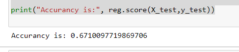

The result is 67 . Not that good let’s get the cross value scores. Cross_val_score is a method which runs cross validation on a dataset to test whether the model can generalise over the whole dataset

Getting the cross val scores

from sklearn.model_selection import cross_val_score

scores = cross_val_score(reg, X_train, y_train, cv=10)
print('Cross-Validation Accuracy Scores', np.mean(scores))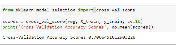

That’s 70 percent. It close but not that good. Let’s improve.

Improving model performance

Here we are fine tuning with grid search method. Grid-search is used to find the optimal hyperparameters of a model which results in the most ‘accurate’ predictions. You can find more info in here.

from sklearn.pipeline import Pipeline
from sklearn.ensemble import RandomForestClassifier
from sklearn.model_selection import GridSearchCV
pipe = Pipeline([('classifier' , RandomForestClassifier())])
# pipe = Pipeline([('classifier', RandomForestClassifier())])

# Create param grid.

param_grid = [
    {'classifier' : [linear_model.LogisticRegression()],
     'classifier__penalty' : ['l1', 'l2'],
    'classifier__C' : np.logspace(-4, 4, 20),
    'classifier__solver' : ['liblinear']},
    {'classifier' : [RandomForestClassifier()],
    'classifier__n_estimators' : list(range(10,101,10)),
    'classifier__max_features' : list(range(6,32,5))}
]

# Create grid search object

reg = GridSearchCV(pipe, param_grid = param_grid, cv = 5, verbose=True, n_jobs=-1)

# Fit on data

reg.fit(X_train, y_train)
print("Accurancy is:", reg.score(X_test,y_test))

scores = cross_val_score(reg, X_train, y_train, cv=10)
print('Cross-Validation Accuracy Scores', np.mean(scores))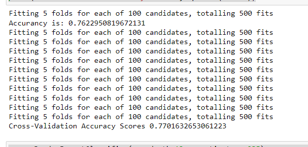

Drawing the confusion matrix

By fitting the RandomForestClassifier model with the default parameters, we have a much ‘better’ model. The accuracy is 77% and at the same time. Now, let’s take a look at the confusion matrix again for this model results again :

from sklearn.metrics import confusion_matrix
y_pred = reg.predict(X_test)
cm = confusion_matrix(y_test,y_pred)
cm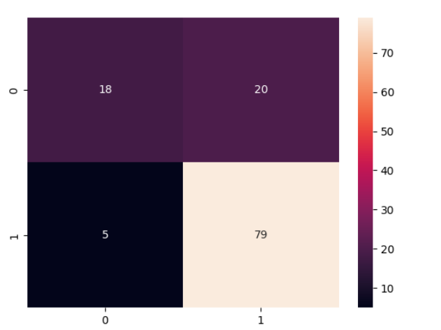

Looking at the misclassified instances, we can observe that 5 malignant cases have been classified incorrectly as benign (False negatives). Also, 20 benign case has been classified as malignant (False positive).

We need a way to minimize the false negatives

A false negative is more serious as it would be that person would not qualify for the loan theorically even if he qualifies. At the same time, a false positive would lead to an unnecessary loan approvals

For achieving this, we would again apply, grid search for tuning hyperparameters.

#Grid Search
from sklearn.metrics import accuracy_score,recall_score,precision_score,f1_score
# X_train, X_test, y_train, y_test 
from sklearn.model_selection import GridSearchCV
clf = LogisticRegression()
grid_values = {'penalty': ['l1', 'l2'],'C':[0.001,.009,0.01,.09,1,5,10,25]}
grid_clf_acc = GridSearchCV(clf, param_grid = grid_values,scoring = 'recall')
grid_clf_acc.fit(X_train, y_train)

#Predict values based on new parameters
y_pred_acc = grid_clf_acc.predict(X_test)

# New Model Evaluation metrics 
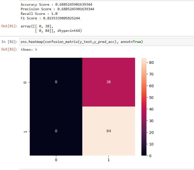
print('Accuracy Score : ' + str(accuracy_score(y_test,y_pred_acc)))
print('Precision Score : ' + str(precision_score(y_test,y_pred_acc)))
print('Recall Score : ' + str(recall_score(y_test,y_pred_acc)))
print('F1 Score : ' + str(f1_score(y_test,y_pred_acc)))

#Logistic Regression (Grid Search) Confusion matrix
confusion_matrix(y_test,y_pred_acc)