Data processing in machine learning is the first one in the bucket for data scientists. Building model getting the accuracy or creating confusion matrix is something which is secondary in context of data. When data is concerned, data analysis is inevitable. And the first step to efficient data analysis is doing a proper data preprocessing in data analytics.
How to do data preprocessing in machine learning
In the post, we will check out data preprocessing steps in data science for a huge data set called “Fintech_dataset”. You can find the jupyter file and data set from here.
So, when you get to large dataset, having industry knowledge is somewhat of great advantage. In that way you will know which features should be of great importance when you are building the model. But since this article is beginner friendly, we have alternative ways to let python do the work for us.
Data preprocessing in machine learning step by step
Step-1 Missing Values
As soon as you get the dataset, after you visualize the data, the first step of data preprocessing in data analytics is doing the below.

This step will tell you how may NaN values are present as a total, and then which column has how many NaN values which you have to get rid of.
For proper data preprocessing in data analytics, its is safe to remove the columns which has all the values as NaN.
The strategy goes like this, take the sum of null value for particular columns, remove which has majority of NaN value and when you find a column where the NaN values are less compared to huge amount you encountered before, then replace it with most frequent values from the column. You can use fillNa function to replace it with frequent values. This is also applicable for categorical values.
Apart from removing columns, which is mainly adopted for continuous numerical values, there are other strategies too.
This again depend on what type of data in time series we are dealing with. While this is a complete different point of interest with its own concepts, I will just shed light on few of the concepts required in our current context of imputing missing values.
There are three categories for data analysis here.
data without trend and without seasonality
Use mean, median, mode or by random sample imputation
data with trend and without seasonality
Use linear interpolation
data with trend and with seasonality
Use seasonal adjustment plus interpolation
This is when there is a gradual increase/decrease in data values as time passes starting from any point in time known as trend.
When a trend repeats itself periodically from time to time known as seasonality
Here is a complete guide of how to visualize trends and seasonality in data.
Apart from this, we have univariate and multivariate imputation.
Univariate imputation implies that we are only considering the values of a single column when performing imputation. Multivariate imputation, on the other hand, involves taking into account other features in the dataset when performing imputation.
For multi-variate we have three ways to treat missing values.
- Simple Imputer
- KNN imputer
- Iterative imputer
Step2 – Outlier Identification
Next step is to identify the outliers and either remove them or replace them with proper constants. Mark this is applicable for continuous variables.
So, the first step to this is detecting the outliers.
Basically, these are the abnormal observations that skew the data distribution, and arise due to inconsistent data entry, or erroneous observations.
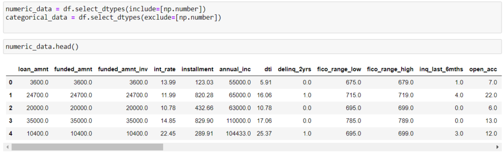
You can visualize the data distribution using a distplot. In order to get into the detection part of outliers, we have to first separate the columns which are numerical as compared to categorical. The code for the same is .
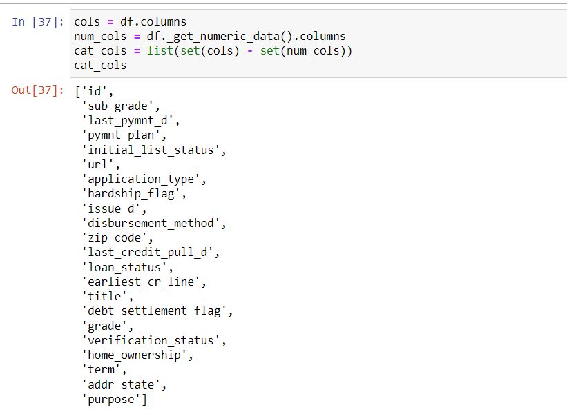
Now we will create a new data frame out of the numerical columns for the outlier detection
Now that we have out target data frame ready, we can look at what are the methods we can use to detect the outliers.
First check what is the distribution type of the data points.
Normal Distribution
Within a group of datapoints, the individual datapoints in normal or gaussian distribution, are symmetric. Their value lies about the mean. This shows that the value near the mean occur more frequently than the values that are farther away from the mean.
Visually it is a bell curve, where most of the data points lie towards the middle of the graph which is the median.
How to detect an outlier for normal distribution? – Use Z score method
You can find more comprehensive explanation on the you tube channel.
- Set up thee upper and lower limit. This will signify that any datapoint outside this range is an outlier
- Upper: Mean + 3 * standard deviation
- Lower: Mean – 3 * standard deviation.
- For python implementation for upper and lower limits are :
- df[‘column’].mean() + 3*df[‘col’].std()
- df[‘column’].mean() – 3*df[‘col’].std()
- Detect how many outliers are present which are not falling in this range
- df[(df[‘column’] > upperlimit) | (df[‘column’] < lowerlimit)]
Further we can apply two techniques of removing the outliers using trimming and capping methods.
How to detect an outlier for skewed distribution? – Use IQR filtering method
We can use box plot to visualize outliers for skewed distribution, and see how many data points are laying outside of the limits.
- Find the Inter Quartile Range (IQR)
- This is the 25th and 75th percentile of the data points
- In python, you can get the above using pandas quantile method
- percentile25 = df[‘column’].quantile(0.25)
- percentile75 = df[‘column’].quantile(0.75)
- The IQR is percentile75 – percentile25
- Formula to calculate the upper limit is percentile75 + 1.5 * IQR
- Formula to calculate the lower limit is percentile25 – 1.5 * IQR
- df[df[‘col’] > upper_limit] – get the data frame to see what are the bad data points
- df[df[‘col’] > upper_limit].count() – to see the count of data points
Further we can apply two techniques of removing the outliers using trimming and capping methods.
Trimming And Capping to treat outliers
With trimming we will be creating one more data frame to have majority of the bad data points removed.
new_df = df[df['col'] < upper_limit]
new_df.shape
So, if you visualize this new data set using box plot, majority of the outliers, would have gotten removed.
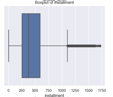
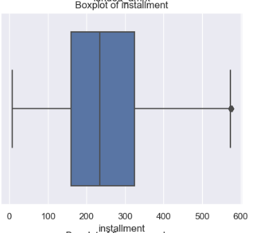
As you could see the change in the data points distribution from above two picture after trimming. There is still a slight spike in the 60-80 segment of the data. This is where we are supposed to apply capping to get rid of the outlier to its fullest.
The code for the same is .
new_df_cap['column'] = np.where(
    new_df ['column'] > upper_limit,
    upper_limit,
    np.where(
        new_df ['column'] < lower_limit,
        lower_limit,
        new_df ['column']
    )
)
Here we are imputing the the valid values to remain in the range of the upper and lower limit that we set using the IQR technique.
After having done with numerical data , its time to proceed with handling the categorical that we created earlier to convert the datapoints to something understandable to the machine while learning. This is the next step of data processing in machine learning.
Step3 – Handling Categorical Data
There are several methods to convert the categorical data to machine understanding language, which is exactly the next step. Here is a sneak peak of what you can follow to understand various techniques for categorical transformations.
For this situation, we are using ‘LabelEncoder’ from sklearn to preprocess categorical data. After that it would look like below.
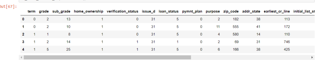
Mark the reason I chose Label encoder is because it’s not going to add extra columns to the data set when already have enough columns. Whereas other methods of encoding like pandas getDummies or one hot encodings would already as much columns as the variations in the properties. This is not good for feeding it to the model.
After having done that we can concatenate the numerical data with the categorical ones to get the final dataset which we can use to train the model.
That was all about data preprocessing in machine learning for a huge data set for fintech. Hope that helped!